PPL SDE
This blog is still under heavy construction.
We look at parameter estimation ofstochastic differential equation models, using the probabilistic programming language Turing. Specifically for a version of the LV model with process noise. We generate the true data.
using Pkg; Pkg.activate("."); Pkg.instantiate()
using DifferentialEquations
using DiffEqNoiseProcess
using Turing
using Distributions
using LinearAlgebra
using Plots, StatsPlots
using Random; Random.seed!(85455)

function lotka_volterra!(du, u, p, t)
    # Model parameters.
    α, β, γ, δ = p
    # Current state.
    x, y = u

    # Evaluate differential equations.
    du[1] = (α - β * y) * x # prey
    du[2] = (δ * x - γ) * y # predator

    return nothing
end
function process_noise!(du, u, p, t)
    du[1] = u[1]*0.025
    du[2] = u[2]*0.025
end
u0 = [1.0, 1.0]

t0,tend = 0,10
measurement_freq = 1.0
noise_freq = 0.1
tspan = (t0,tend)
tmeasure = tend/2:measurement_freq:tend
tgrid = t0:noise_freq:tend
p = [1.5, 1.0, 3.0, 1.0]
W = WienerProcess(0.0, zeros(length(u0)))
prob = SDEProblem(lotka_volterra!,process_noise!,u0,tspan,p,saveat=tmeasure,noise=W)

sol = solve(prob,saveat=[],reltol=1e-6,abstol=1e-6)
plot(sol)
scatter!(sol(tmeasure))
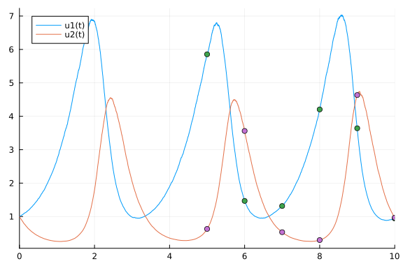
data = sol(tmeasure)[:,:]
data_vec  = reshape(data,length(u0)*(length(tmeasure)))
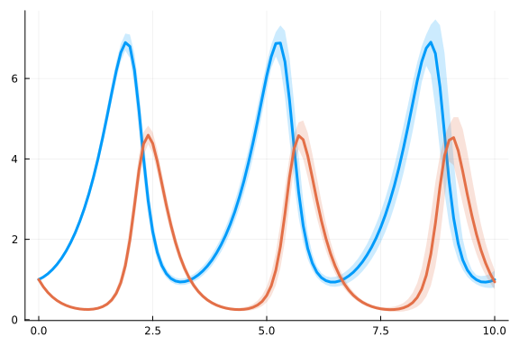
Let us look at an ensemble of possible solutions with the same parameters.
ensembleprob = EnsembleProblem(prob)
ensemblesol = solve(ensembleprob,EnsembleThreads(),trajectories=1000,saveat=t0:0.1:tend,reltol=1e-6,abstol=1e-6)
ensemblesumm = EnsembleSummary(ensemblesol)
plot(ensemblesumm)

The SDE solvers discretize the process noise in time.
However, by default the SDE solvers are adaptive, and thus evaluate the process noise,
at different time-points for each solve. Turing can, however, only perform inference if
in each step if the amount of random variables and their meaning
is the same in each iteration of the MC-MC algorithm.
StochasticDifferentialEquations.jl allows you to provide an already discretized
version of the process noise to the solver using NoiseGrid.
The the price you pay is that the process noise is interpolated linearly
between the grid points, which is less accurate than if you let the solver chose its own
discretization of the stochastic process (see Brownian bridge).
function prob_func(prob,i,repeat)
    brownian_noise = rand(MvNormal(zeros(length(u0)*(length(tgrid)-1)),noise_freq*I))
    brownian_noise = reshape(brownian_noise,length(u0),length(tgrid)-1)
    brownian_noise = vcat([zeros(length(u0))], [c for c in eachcol(brownian_noise)])
    W = NoiseGrid(vcat(tgrid,10.1),vcat(cumsum(brownian_noise),[rand(length(u0))]))
    remake(prob,noise=W)
end
ensembleprob = EnsembleProblem(prob,prob_func=prob_func)
ensemblesol = solve(ensembleprob,EnsembleThreads(),trajectories=1000,saveat=t0:0.1:tend,reltol=1e-6,abstol=1e-6)
ensemblesumm = EnsembleSummary(ensemblesol)
plot(ensemblesumm)
Now let us do inference using the Metropolis-Hastings algorithm.
@model function model(data_vec, prob)
tmeasure = prob.kwargs[:saveat]
u0 = prob.u0
# Prior distributions for parameters of interest
p1 ~ Uniform(0.5,3.5)
p2 ~ Uniform(0.5,3.5)
p3 ~ Uniform(0.5,3.5)
p4 ~ Uniform(0.5,3.5)
p = [p1,p2,p3,p4]
# Prior distribution for process noise measurement times
brownian_noise ~ MvNormal(zeros(length(u0)*(length(tgrid)-1)),noise_freq*I)
brownian_noise = reshape(brownian_noise,length(u0),length(tgrid)-1)
brownian_noise = vcat([zeros(length(u0))], [c for c in eachcol(brownian_noise)])
W = NoiseGrid(vcat(tgrid,10.1),vcat(cumsum(brownian_noise),[rand(length(u0))]))
# simulating the system
prob = remake(prob,p=p,noise=W)
sol = solve(prob,reltol=1e-6,abstol=1e-6)
failure = size(sol, 2) < length(tmeasure)
if failure
println("failure")
Turing.DynamicPPL.acclogp!!(__varinfo__, -Inf)
return
end
# likelihood
sol_vec = reshape(sol[:,:],length(u0)*(length(tmeasure)))
data_vec ~ MvNormal(sol_vec,0.01^2*I)
return nothing
end
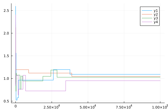
chain = sample(model(data_vec, prob), MH(), MCMCThreads(), 100_000, 4)
plot(chain[:p1])
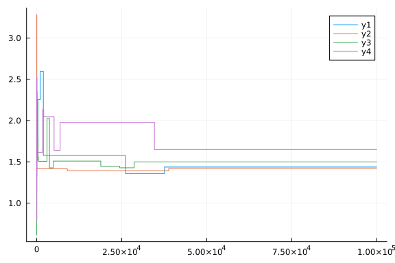
plot(chain[:p2])
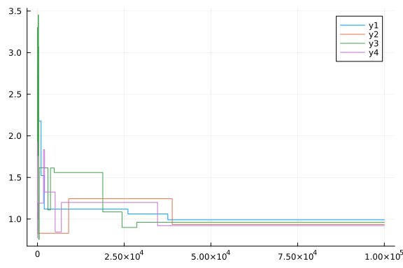
plot(chain[:p3])
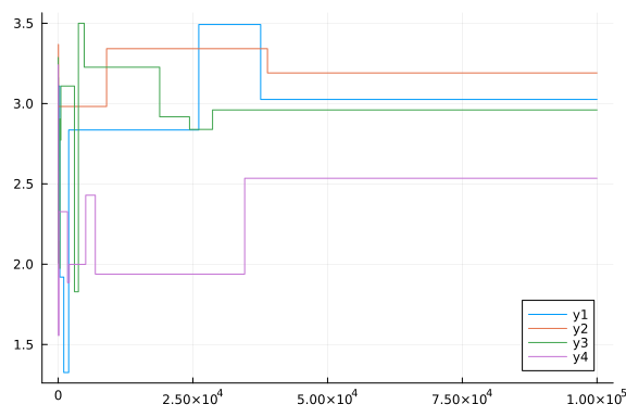
plot(chain[:p4])