Design for model discrimination using symbolic regression
Most experimental design focusses on parameter precision, where the model structure is assumed known and fixed. But arguably finding the correct model structure is the part of the modelling process that takes the most effort. In this blog we will look at automating this process using symbolic regression, and to do this with gathering too much data.
The Julia packages that we will use:
using SymbolicRegression
using Symbolics, SymbolicUtils
using Distributions
using Optimization, OptimizationBBO
using Plots
using Random; Random.seed!(12345)
We will try to discover the equation: $$y(x) = \exp(-x)\sin(2\pi x) + \cos(\frac{\pi}{2}x), \qquad 0 \leq x \leq 10,$$ automatically from data. Translated into Julia code:
y(x) = exp(-x)*sin(2π*x) + cos(π/2*x)
y(0.0)
1.0
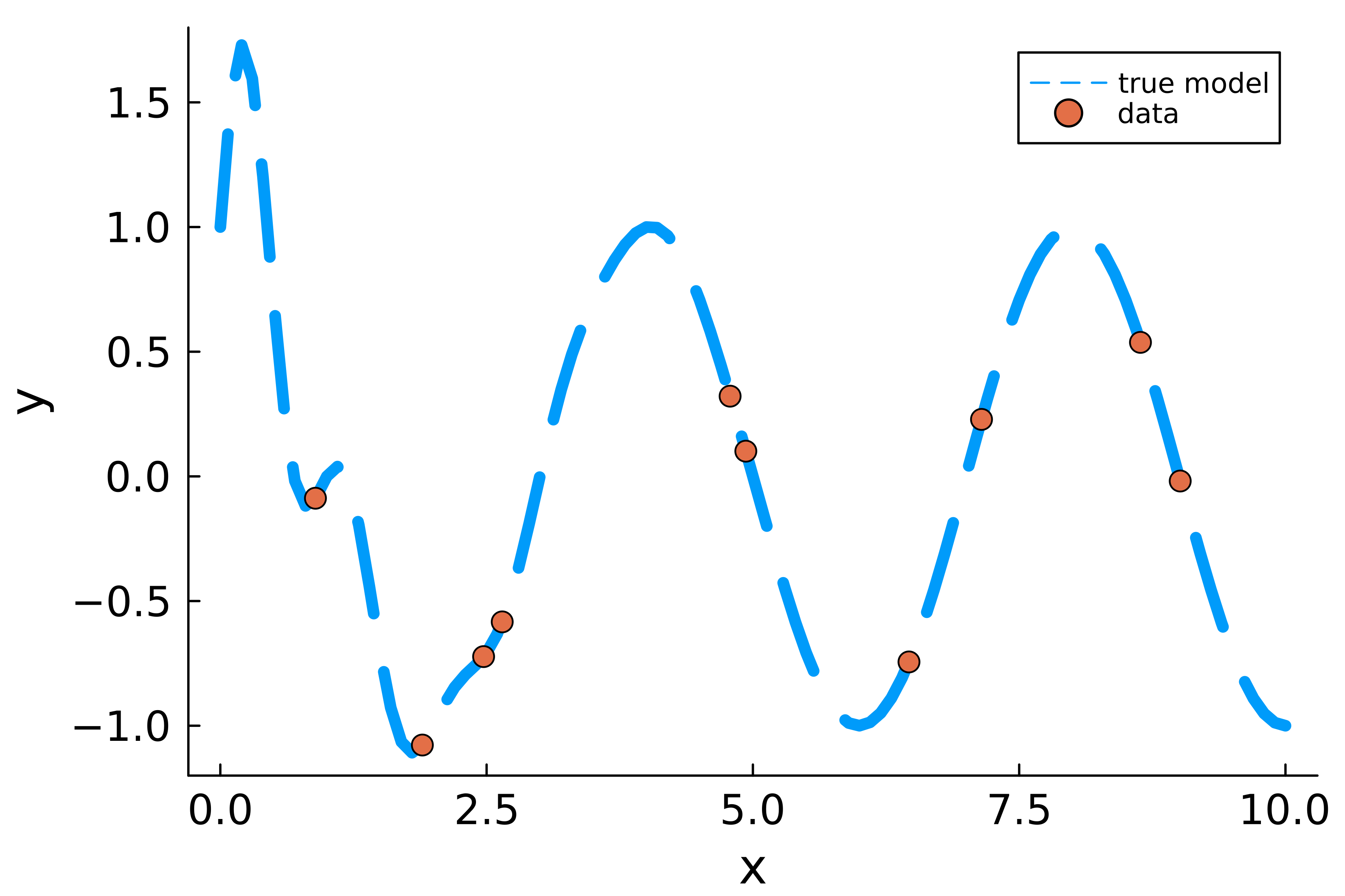
As a baseline design let us gather 10 points randomly from the design space.
n_obs = 10
design_region = Uniform(0.0,10.0)
X = rand(design_region,n_obs)
Y = y.(X)
plot(0.0:0.1:10.0,y.(0.0:0.1:10.0),label="true model",lw=5,ls=:dash);
scatter!(X,Y,ms=5,label="data");
plot!(xlabel="x",ylabel="y", ylims=(-1.2,1.8));
plot!(tickfontsize=12, guidefontsize=14, legendfontsize=8, grid=false, dpi=600)
Now let us perform symbolic regression on this dataset. We will look for 10 model structures that fit the data.
options = SymbolicRegression.Options(
    unary_operators = (exp, sin, cos),
    binary_operators=(+, *, /, -),
    seed=123,
    deterministic=true
)
hall_of_fame = EquationSearch(X', Y, options=options, niterations=100, runtests=false, parallelism=:serial)
n_best_max = 10
#incase < 10 model structures were returned
n_best = min(length(hall_of_fame.members),n_best_max)
best_models = sort(hall_of_fame.members,by=member->member.loss)[1:n_best]
Started!
10-element Vector{SymbolicRegression.PopMemberModule.PopMember{Float64}}:
 SymbolicRegression.PopMemberModule.PopMember{Float64}((cos(x1 * -1.5707472
736173678) - sin(sin(exp(x1) / cos(sin((x1 * 0.11489592239489567) + 0.02924
150694094207))) / exp(x1))), 0.06403884841950626, 1.0187179197773552e-5, 24
01441, 5807529618927081144, 5795836981119531379)
 SymbolicRegression.PopMemberModule.PopMember{Float64}((cos(x1 * -1.5707472
736173678) - (sin(exp(x1) / cos(sin((x1 * 0.11489592239489567) + 0.02924150
694094207))) / exp(x1))), 0.06083908652153372, 1.0249160815942009e-5, 20897
28, 4358865566510575018, 1198926568467179219)
 SymbolicRegression.PopMemberModule.PopMember{Float64}((cos(x1 / 0.63660506
56890262) - sin(sin(exp(x1) / cos(sin(0.11489592239489567) * x1)) / exp(x1)
)), 0.057681573488650405, 2.1388759091569173e-5, 1738646, 35215362873834417
13, 1106443898740131553)
 SymbolicRegression.PopMemberModule.PopMember{Float64}((cos(x1 / 0.63660506
56890262) - sin(sin(exp(x1) / cos(0.11489592239489567 * x1)) / exp(x1))), 0
.054481940153208334, 2.148542646434505e-5, 1683449, 1106443898740131553, 44
63609806790343470)
 SymbolicRegression.PopMemberModule.PopMember{Float64}((cos(x1 / 0.63660506
56890262) - (sin(exp(x1) / cos(0.11489592239489567 * x1)) / exp(x1))), 0.05
1288010332056364, 2.3076573687286177e-5, 1458762, 4463609806790343470, 2723
675212815722575)
 SymbolicRegression.PopMemberModule.PopMember{Float64}((cos(x1 / 0.63660506
56890262) - (sin(exp(x1) * 1.0363388900284802) / (exp(x1) - 0.1934422901771
7546))), 0.04817556182698313, 4.603205300197051e-5, 2412019, 50722280559235
5699, 4112726823019557294)
 SymbolicRegression.PopMemberModule.PopMember{Float64}((cos(x1 / 0.63660506
56890262) - (sin(exp(x1) * 1.0363388900284802) / exp(x1))), 0.0419268037121
5973, 8.568762695441023e-5, 1359344, 682475129147039269, 320765785728912140
4)
 SymbolicRegression.PopMemberModule.PopMember{Float64}((cos(x1 / 0.63660506
56890262) - (sin(exp(x1) / cos(0.28864399612143354)) / exp(x1))), 0.0451293
8764414751, 8.636558026583333e-5, 2581722, 6623397325472061777, 38276093791
68211583)
 SymbolicRegression.PopMemberModule.PopMember{Float64}((cos(x1 * -1.5707472
736173678) - (sin(sin(exp(x1))) / exp(x1))), 0.03946124078956312, 0.0002782
5693509305236, 1189722, 6591081748771200099, 1673930060287288728)
 SymbolicRegression.PopMemberModule.PopMember{Float64}((cos(x1 * -1.5707472
736173678) - (sin(exp(x1)) / exp(x1))), 0.036415945717573416, 0.00031881998
770847704, 1123566, 4441784085260582951, 8874312346525345533)
TECHNICAL NOTE: I ordered the model structures purely by mean squared error loss of the fits. Symbolic regression usually also incorporates a punishment for complexity of the model. I did not yet find a good way to incorporate this in the experimental design workflow, but this is definitely something that should be looked at.
Now let us turn these symbolic expressions back into executable functions. Let us try it for the first suggested model structure:
@syms x
eqn = node_to_symbolic(best_models[1].tree, options,varMap=["x"])
cos(-1.5707472736173678(x^1)) - sin(sin(exp(x) / cos(sin(0.0292415069409420
7 + 0.11489592239489567x))) / exp(x))
using SymbolicUtils.Code
func = Func([x],[],eqn)
expr = toexpr(func)
_f = build_function(eqn,x)
:(function (x,)
      #= C:\Users\arno\.julia\packages\SymbolicUtils\qulQp\src\code.jl:349
=#
      #= C:\Users\arno\.julia\packages\SymbolicUtils\qulQp\src\code.jl:350
=#
      #= C:\Users\arno\.julia\packages\SymbolicUtils\qulQp\src\code.jl:351
=#
      (-)((cos)((*)(-1.5707472736173678, (^)(x, 1))), (sin)((/)((sin)((/)((
exp)(x), (cos)((sin)((+)(0.02924150694094207, (*)(0.11489592239489567, x)))
))), (exp)(x))))
  end)
f = eval(_f)
f.(X)
10-element Vector{Float64}:
  0.22766738661929953
 -0.08666167715710274
  0.5377339408803581
 -0.018287438097402808
 -0.7453936527293958
 -1.069802392904377
  0.32276595996282476
 -0.5786714569337166
 -0.7262625548623343
  0.09948952933242539
Now we do it for all the others and plot them:
plot(0.0:0.1:10.0,y.(0.0:0.1:10.0),lw=5,label="true model",ls=:dash);
model_structures = Function[]
for i = 1:n_best
    eqn = node_to_symbolic(best_models[i].tree, options,varMap=["x"])
    fi = eval(build_function(eqn,x))
    x_plot = Float64[]
    y_plot = Float64[]
    for x_try in 0.0:0.1:10.0
        try
            y_try = fi(x_try)
            append!(x_plot,x_try)
            append!(y_plot,y_try)
        catch
        end
    end
    plot!(x_plot, y_plot,label="model $i");
    push!(model_structures,fi)
end
scatter!(X,Y,ms=5,label="data",ls=:dash);
plot!(xlabel="x",ylabel="y", ylims=(-1.2,1.6));
plot!(tickfontsize=12, guidefontsize=14, legendfontsize=8, grid=false, dpi=600)
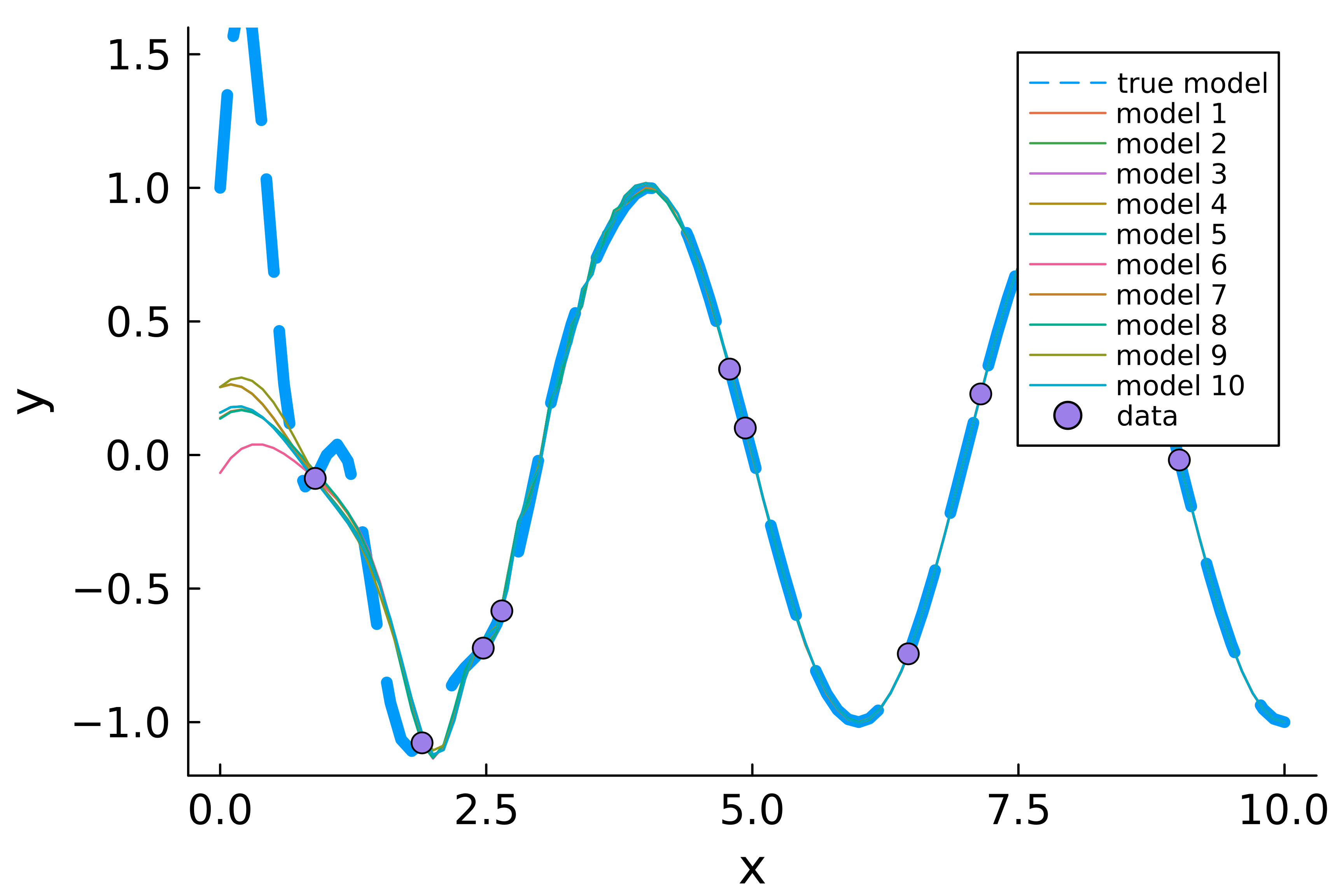
We see that none of the suggested model structures approximate the true model well in the area between $0$ and $2.5$, while between $2.5$ and $10$ the models agree. In this case it is thus probably a good idea to gather more data for small $x$. Can we formalize this in mathematical terms? We will do this by creating a variant of T-optimal designs. T-optimal designs are model discrimination designs, where design points are sought which maximize the distance between a model thought to be correct (T for true) and some other plausible alternative model structures. Though perhaps it is better to think of the “true” model as a null hypothesis model. Design points are chosen such that the alternative models predict different values than the “true” model at these points. If the “true” model is then not correct after all, it should be easily discernible from the data.
In our situation, we do not have a model structure which can serve as the “true” model. We will instead work with all pairwise distances between the plausible model structures suggested by symbolic regression. Collecting measurements where the model structures differ greatly in predictions, will cause atleast some of the model structures to become unlikely, causing new model structures to enter the top $10$. We call this S-optimal, with S for Symbolics. $$N = \text{number of measurements}$$ $$M = \text{number of models}$$ $$f_i = \text{ith model structure}$$ $$x_k = \text{kth design point}$$
$$\max_x \frac{2}{M(M-1)}\sum_{i=1}^{N}\sum_{j=i+1}^{N} \max_{k=1 \text{ to } M}\set{(f_i(x_k) - f_j(x_k))^2}$$
TECHNICAL NOTE: The average over the pairwise model comparisons could be replaced with the minimum. This would lead to a max-min-max strategy instead of a max-expected-max strategy. In my experiments this did not work well when two of the suggested model structures are very similar or identical. This often occurs because of terms like $sin(x-x)$ being present in symbolic regression. Punishing for complexity might remedy this.
Now let us apply this criterion to gather $3$ new measurements:
function S_criterion(x,model_structures)
    n_structures = length(model_structures)
    n_obs = length(x)
    if length(model_structures) == 1
        # sometimes only a single model structure comes out of the equation search
        return 0.0
    end
    y = zeros(n_obs,n_structures)
    for i in 1:n_structures
        y[:,i] .= model_structures[i].(x)
    end
    squared_differences = Float64[]
    for i in 1:n_structures
        for j in i+1:n_structures
            push!(squared_differences, maximum([k for k in (y[:,i] .- y[:,j]).^2]))
        end
    end
    -mean(squared_differences) # minus sign to minimize instead of maximize
end
function S_objective(x_new,(x_old,model_structures))
    S_criterion([x_old;x_new],model_structures)
end
n_batch = 3
X_new_ini = rand(design_region,n_batch)
S_objective(X_new_ini,(X,model_structures))
-0.015370296718503698
TECHNICAL NOTE: Can this be reformulated as a differentiable optimization problem, using slack variables?
lb = fill(minimum(design_region),n_batch)
ub = fill(maximum(design_region),n_batch)
prob = OptimizationProblem(S_objective,X_new_ini,(X,model_structures),lb = lb, ub = ub)
X_new = solve(prob,BBO_adaptive_de_rand_1_bin_radiuslimited(),maxtime=10.0)
u: 3-element Vector{Float64}:
 1.867790602985872e-18
 0.22833800197426193
 3.301026120902155
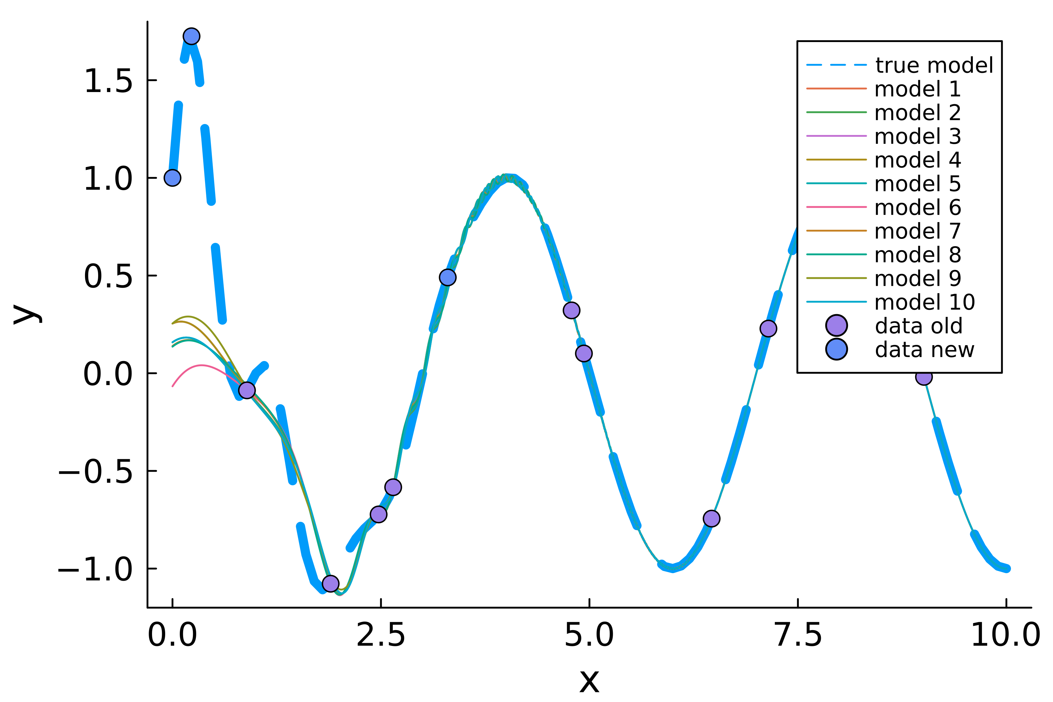
We see that $2$ new observations are indeed both smaller than $2.5$. The last one is used to discriminate between two models that are almost indistinguishable with the naked eye. Let us plot this:
Y_new = y.(X_new)
plot(0.0:0.1:10.0,y.(0.0:0.1:10.0),lw=5,label="true model",ls=:dash);
for i = 1:n_best
    x_plot = Float64[]
    y_plot = Float64[]
    for x_try in 0.0:0.01:10.0
        try
            y_try = model_structures[i](x_try)
            append!(x_plot,x_try)
            append!(y_plot,y_try)
        catch
        end
    end
    plot!(x_plot, y_plot,label="model $i");
end
scatter!(X,Y,ms=5,label="data old");
scatter!(X_new,Y_new,ms=5,label="data new");
plot!(xlabel="x",ylabel="y", ylim=(-1.2,1.8));
plot!(tickfontsize=12, guidefontsize=14, legendfontsize=8, grid=false, dpi=600)
Now, we run symbolic regression on our combined dataset:
X = [X;X_new]
Y = [Y;Y_new]
hall_of_fame = EquationSearch(X', Y, options=options, niterations=100, runtests=false, parallelism=:serial)
n_best = min(length(hall_of_fame.members),n_best_max)
best_models = sort(hall_of_fame.members,by=member->member.loss)[1:n_best]
plot(0.0:0.01:10.0,y.(0.0:0.01:10.0),lw=5,label="true model",ls=:dash);
model_structures = Function[]
for i = 1:n_best
    eqn = node_to_symbolic(best_models[i].tree, options,varMap=["x"])
    println(eqn)
    fi = eval(build_function(eqn,x))
    x_plot = Float64[]
    y_plot = Float64[]
    for x_try in 0.0:0.01:10.0
        try
            y_try = fi(x_try)
            append!(x_plot,x_try)
            append!(y_plot,y_try)
        catch
        end
    end
    plot!(x_plot, y_plot,label="model $i");
    push!(model_structures,fi)
end
scatter!(X,Y,ms=5,label="data");
plot!(xlabel="x",ylabel="y", ylims=(-1.2,1.8));
plot!(tickfontsize=12, guidefontsize=14, legendfontsize=8, grid=false, dpi=600)
Started!
cos(1.5707963267136822(x^1)) - (sin(-6.283185306231179(x^1)) / exp(x))
cos(1.5707963267136822(x^1)) - (sin(-6.283185306231179(x^1)) / exp(x))
cos(1.5707963267136822(x^1)) - (sin((x^1)*((-5.283185306231179 - cos(x - x)
)^1)) / exp(x))
cos(1.5707963267136822(x^1)) - (sin((x^1)*((-5.283185306231179 - exp(1.5707
963267136822((x - x)^1)))^1)) / exp(x))
cos(1.5707963267136822(x^1)) - (sin((-5.283185306231179(x^1)) - x) / exp(x)
)
cos(1.5707963267136822(x^1)) - (sin(((-5.283185306231179 / x)*(x^2)) - x) /
 exp(x))
cos(1.5707963267136822(x^1)) - (sin(((sin(x) - 5.283185306231179x) - x) - s
in(x)) / exp(x))
cos(1.5707963265959193(x^1)) - (sin(x / -0.15915494382513268) / exp(x))
cos(1.5707768686144095(x^1)) - (sin(x / -0.1589621029216852) / exp(x))
cos(1.571732202757438(x^1)) - sin(0.2460674037875204 / (x*x))
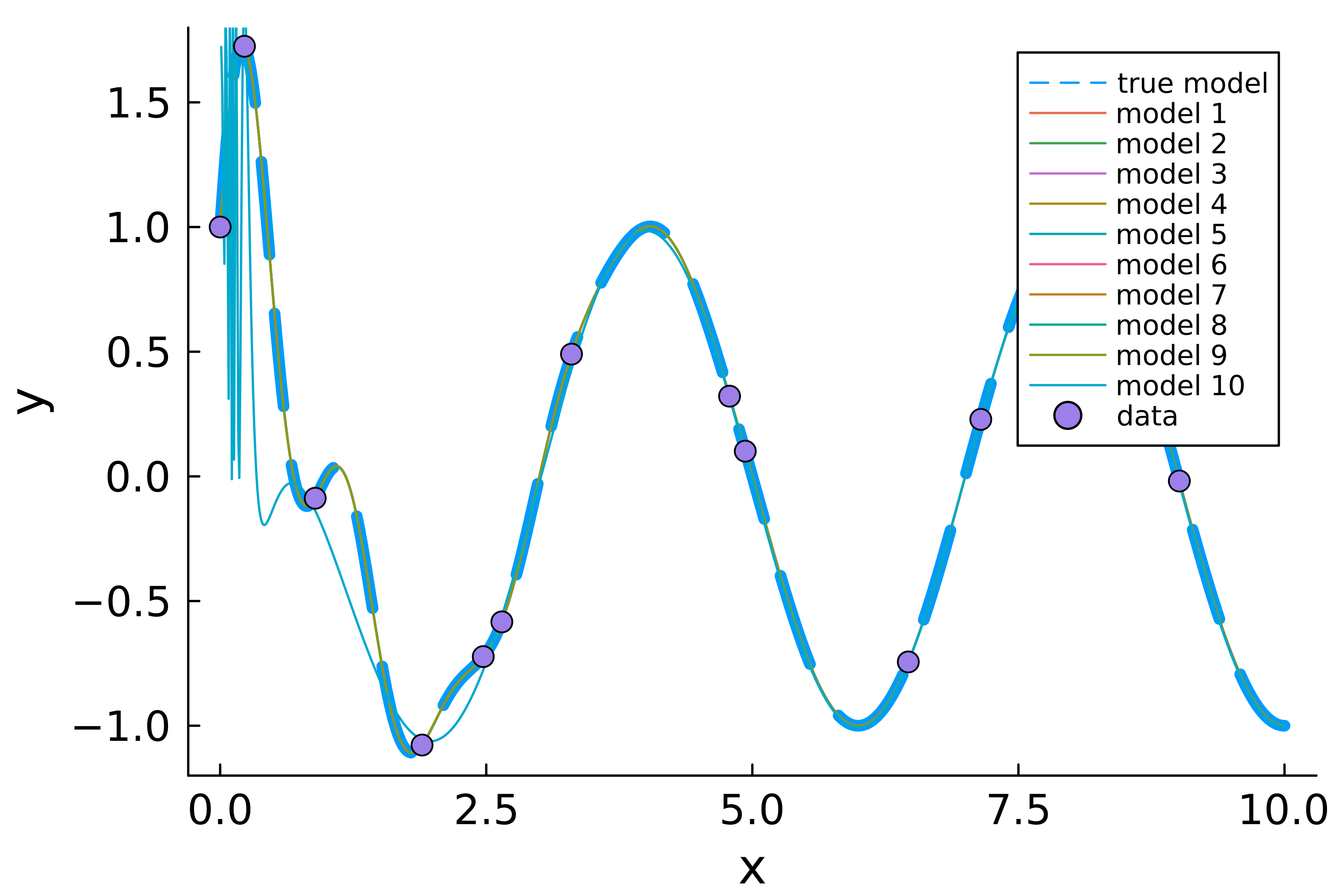
Et voilà, we found the correct model structure, with only 3 new observations!
TECHNICAL NOTE: In fact we found it multiple times, with expressions like $sin(x-x)$. Again, punishing for needless complexity would be of added value here.